Tutorials
Learn More
Carry Look Ahead Adder
The drawback of ‘Ripple carry adder‘ is that it has a carry propagation delay that introduces slow computation. Since adders are used in designs like multipliers and divisions, it causes slowness in their computation. To tackle this issue, a carry look-ahead adder (CLA) can be used that reduces propagation delay with additional hardware complexity.
CLA has introduced some functions like ‘carry generate (G)’ and ‘carry propagate (P)’ to boost the speed.
Carry Generate (G): This function denotes how the carry is generated for single-bit two inputs regardless of any input carry.
As we have seen in the full adder, carry is generated using the equation as A.B.
Hence, G = A·B (similar to how carry is generated by full adder)
Carry Propagate (P): This function denotes when the carry is propagated to the next stage with an addition whenever there is an input carry.
Let’s consider single bit two inputs A and B.
|
A |
B |
Carry In |
Description |
|
0 |
0 |
1 |
Carry is not propagated (0) |
|
0 |
1 |
1 |
Carry is propagated (1) |
|
1 |
0 |
1 |
Carry is propagated (1) |
|
1 |
1 |
1 |
Carry is propagated (1) |
Thus, P = A+B
Carry computation function for next stage
Cj+1 = Gj+(Pj·Cj)
= Aj·Bj + (Aj + Bj)·Cj
However, if you notice clearly whenever Aj=1 and Bj=1
Cj+1 = 1 (always) as Aj·Bj component nullifies effect of [(Aj + Bj)·Cj] part. Thus, it does not matter even if you use the equation propagate function as P = A (+) B as mentioned in other literature.
G = A·B
P = A + B or A (+) B
Block Diagram
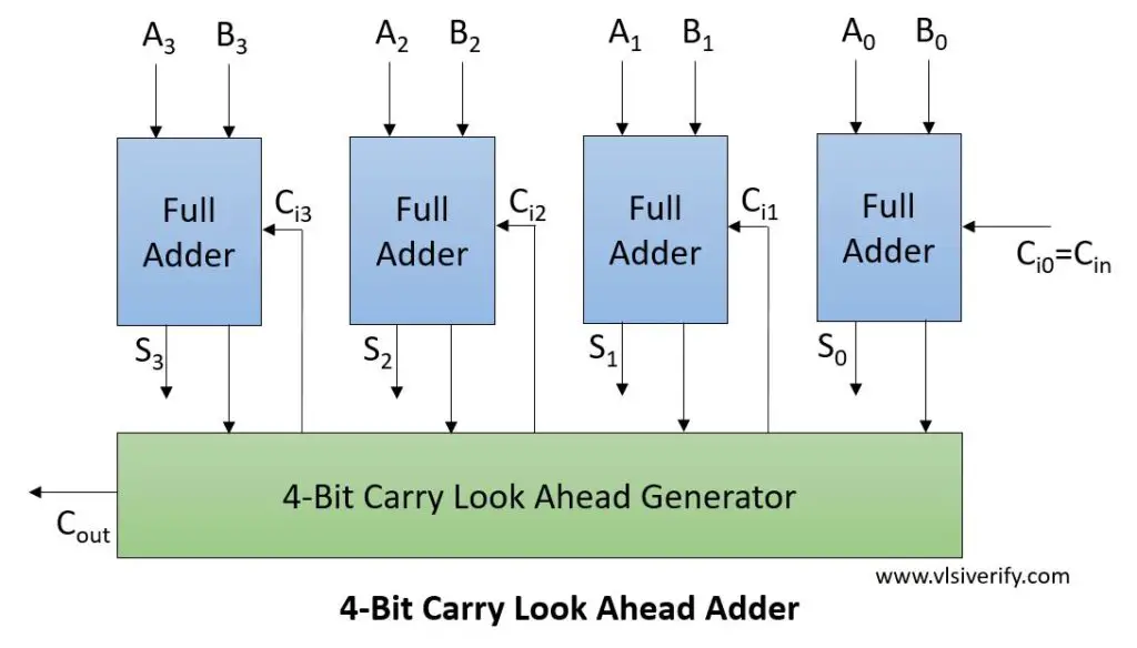
Computation of all carry for next stage addition
Inputs –
A3 A2 A1 A0
B3 B2 B1 B0
And Cin
Output
Sum = S3 S2 S1 S0
And Cout
Sum Sj = Pj ^ Cj = Aj ^ Bj ^ Cj
C0 = Cin
C1 = G0 + (P0·C0)
= A0·B0 + (A0^B0)·C0
C2 = G1 + (P1·C1)
= A1·B1 + (A1^B1)·(A0·B0 + (A0^B0)·C0)
C3 = G2 + (P2·C2)
= A2·B2 + (A2^B2)·C2
= A2·B2 + (A2^B2)·(A1.B1 + (A1^B1)·(A0B0 + (A0^B0)·C0))
C4 = G3 + (P3·C3)
= A3·B3 + (A3^B3)·C3
= A3·B3 + (A3^B3)·(A2.B2 + (A2^B2)·(A1.B1 + (A1^B1)·(A0B0 + (A0^B0)·C0)))
Cout = C4;
Notice that in each stage we are ultimately dependent on inputs A, B, and Cin. This actually makes it faster as compared to the ripple carry adder which is highly dependent on the carry generated from the previous stage.
The final implementation is brought down to XOR, AND, and OR gate level.
Disadvantage
Requires complex hardware to generate the carry based on input signals and the complexity grows with an increasing number of bits.
Advantage
It does not need to wait till the previous stage generates the carry. It can generate carry for each full adder simultaneously, hence it is faster as compared to the ripple carry adder.
Carry Look Ahead Adder
module CarryLookAheadAdder(
  input [3:0]A, B,
  input Cin,
  output [3:0] S,
  output Cout
);
  wire [3:0] Ci; // Carry intermediate for intermediate computation

  assign Ci[0] = Cin;
  assign Ci[1] = (A[0] & B[0]) | ((A[0]^B[0]) & Ci[0]);
  //assign Ci[2] = (A[1] & B[1]) | ((A[1]^B[1]) & Ci[1]); expands to
  assign Ci[2] = (A[1] & B[1]) | ((A[1]^B[1]) & ((A[0] & B[0]) | ((A[0]^B[0]) & Ci[0])));
  //assign Ci[3] = (A[2] & B[2]) | ((A[2]^B[2]) & Ci[2]); expands to
  assign Ci[3] = (A[2] & B[2]) | ((A[2]^B[2]) & ((A[1] & B[1]) | ((A[1]^B[1]) & ((A[0] & B[0]) | ((A[0]^B[0]) & Ci[0])))));
  //assign Cout  = (A[3] & B[3]) | ((A[3]^B[3]) & Ci[3]); expands to
  assign Cout  = (A[3] & B[3]) | ((A[3]^B[3]) & ((A[2] & B[2]) | ((A[2]^B[2]) & ((A[1] & B[1]) | ((A[1]^B[1]) & ((A[0] & B[0]) | ((A[0]^B[0]) & Ci[0])))))));

  assign S = A^B^Ci;
endmodule
Testbench Code
module TB;
  reg [3:0]A, B;
  reg Cin;
  wire [3:0] S;
  wire Cout;
  wire[4:0] add;

  CarryLookAheadAdder cla(A, B, Cin, S, Cout);

  assign add = {Cout, S};
  initial begin
    $monitor("A = %b: B = %b, Cin = %b --> S = %b, Cout = %b, Addition = %0d", A, B, Cin, S, Cout, add);
    A = 1; B = 0; Cin = 0; #3;
    A = 2; B = 4; Cin = 1; #3;
    A = 4'hb; B = 4'h6; Cin = 0; #3;
    A = 5; B = 3; Cin = 1;
  end
endmodule
Output:
A = 0001: B = 0000, Cin = 0 --> S = 0001, Cout = 0, Addition = 1
A = 0010: B = 0100, Cin = 1 --> S = 0111, Cout = 0, Addition = 7
A = 1011: B = 0110, Cin = 0 --> S = 0001, Cout = 1, Addition = 17
A = 0101: B = 0011, Cin = 1 --> S = 1001, Cout = 0, Addition = 9
Verilog Codes